带你入门数据处理Chapter 2

Chapter 2: Mastering Data Processing - From Statistics to Feature Engineering

书接上回

Welcome back to my data analytics blog! In this post, I gonna dive deep into Chapter 2 of Beijing Normal-Hong Kong Baptist University’s course materials, focusing on practical data processing skills—from calculating basic statistics to crafting powerful features gogogo 出发喽！

Contents

1. Basic Descriptive Statistics（基础描述性统计）
   1. Key Metrics & Calculation Steps
2. Visualization（数据可视化）
   1. How to Plot Core Charts
   2. Properties of Common Plots
3. Data Cleaning（数据清洗）
   1. Types of Missing Values（缺失值类型）
   2. Outliers: Definition & Detection（异常值：定义与检测）
   3. Handling Outliers & Missing Values（异常值与缺失值处理）
   4. Data Normalization（数据归一化）
4. Feature Selection & Engineering（特征选择与特征工程）
   1. Feature Selection / Dimensionality Reduction（特征选择/降维）
   2. Feature Engineering Techniques（特征工程技术）

---

Basic Descriptive Statistics (基础描述性统计)

Descriptive statistics are the foundation of understanding your data—they summarize key characteristics without making predictions. Below’s how to calculate core metrics for any sequence of numbers.

Key Metrics & Calculation Steps

Let’s use a sample dataset for practice:

1. Mean (均值), Mode (众数), Standard Deviation (标准差)

• Mean (均值): Average of all values.
  • Formula:
  • Calculation:
• Mode (众数): Most frequently occurring value.
  • Calculation: Count occurrences of each value → 85 appears 3 times (mode = 85).
• Standard Deviation (标准差): Measures data spread around the mean (square root of variance).
  • Step 1: Calculate variance
    • Example:
  • Step 2: Take the square root →

2. Median (中位数), 1Q (第一四分位数), 3Q (第三四分位数), IQR (四分位距), Range (极差)

First, sort the dataset: (n=10, even)

• Median (中位数): Middle value (50% quantile).
  • For even n: Mean of the two middle values →
  • For odd n: The middle value directly.
• 1Q (1st Quartile, 第一四分位数): Value where 25% of data is smaller.
  • Step 1: Calculate (not an integer → round up to 3).
  • Step 2: The 3rd value in the sorted dataset → 78.
• 3Q (3rd Quartile, 第三四分位数): Value where 75% of data is smaller.
  • Step 1: Calculate (round up to 8).
  • Step 2: The 8th value in the sorted dataset → 90.
• IQR (Interquartile Range, 四分位距): Range of the middle 50% of data.
  • Formula:
• Range (极差): Difference between max and min values.
  • Formula:

Visualization (数据可视化)

Visualization turns raw data into actionable insights. Below’s how to plot key charts and their core properties.

How to Plot Core Charts

1. Scatter Plot (散点图)

• Purpose: Show relationships between two numerical attributes (e.g., petal length vs. width in Iris data).
• Steps:
  1. Assign one variable to the x-axis and the other to the y-axis.
  2. Plot each data point as a dot.
  3. For large datasets (n > 10,000), use hexagonal binning (六边形分箱) to avoid overcrowding.

Justin Zhang_2025-12-31_00-26-48.png

Justin Zhang_2025-12-31_00-27-09.png

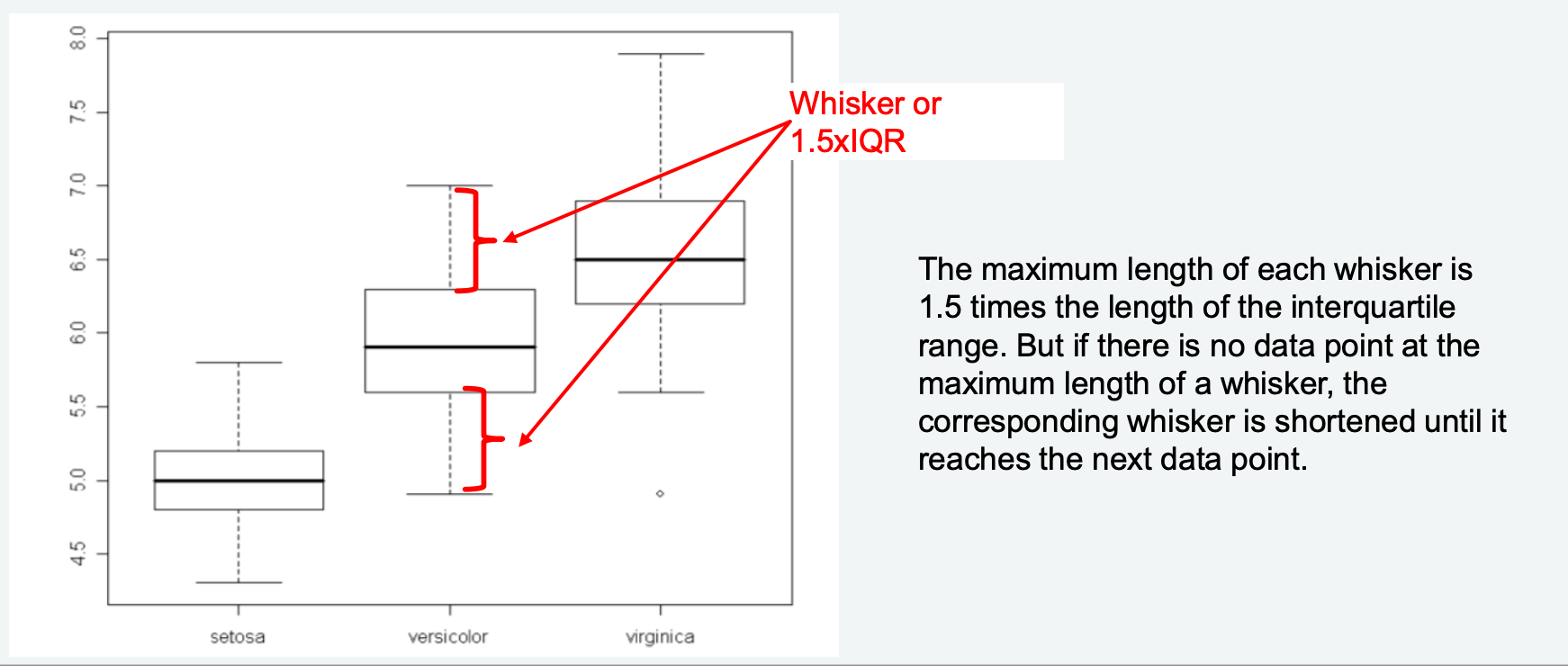
2. Boxplot with Quantiles & Whiskers (带分位数和须的箱线图)

• Purpose: Summarize numerical data (median, IQR, outliers).
• Steps:
  1. Calculate 1Q, Median, 3Q, and IQR.
  2. Draw a box from 1Q to 3Q (contains 50% of data).
  3. Add a line inside the box for the median.
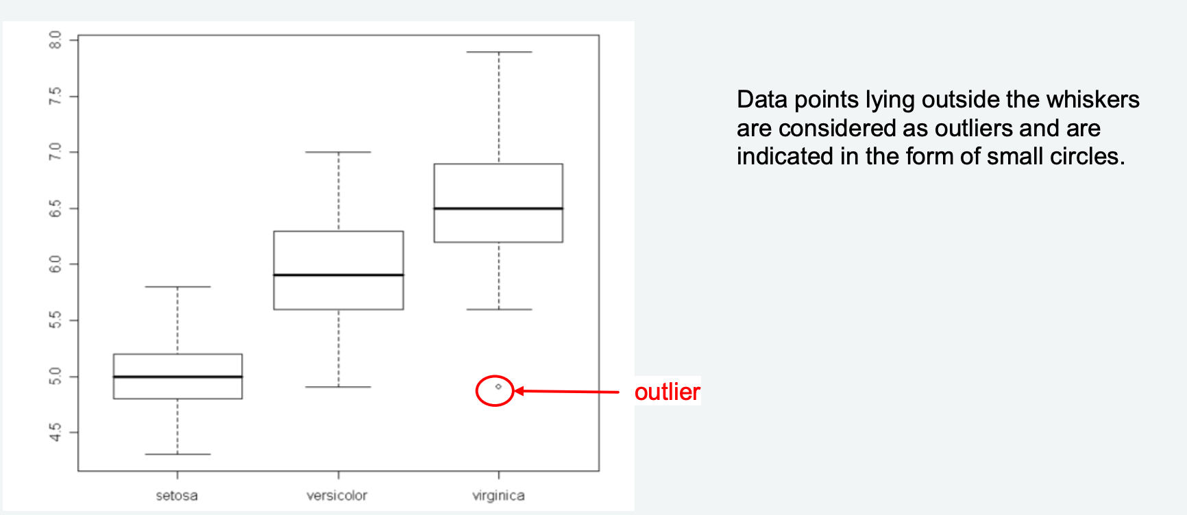
  4. Extend whiskers to the farthest data points within from 1Q/3Q.
  5. Plot outliers (points outside whiskers) as small circles.

Justin Zhang_2025-12-31_00-21-21.png

3. Bar Chart (柱状图)

• Purpose: Compare frequencies of categorical attributes (e.g., game genre popularity).

Justin Zhang_2025-12-31_00-16-35.png

• Steps:
  1. Assign categories to the x-axis and frequencies to the y-axis.
  2. Draw rectangular bars where height = frequency of each category.

Properties of Common Plots

Plot Type (图表类型)	Core Properties (核心属性)
Scatter Plot (散点图)	- Shows correlation between two numerical variables. - Not suitable for large datasets (use hexagonal binning). - Can be enhanced with color/shape to represent third variables.
Pie Plot (饼图)	- Displays the contribution of each category to a total. - Only for single-dimensional categorical data. - Avoid more than 5 categories (hard to read).
Bar Chart / Histogram (柱状图/直方图)	- Bar Chart: For categorical data (distinct bars). - Histogram: For numerical data (continuous bins). - Histogram bin count follows Sturge’s Rule: .
Boxplot (箱线图)	- Compact summary of median, IQR, and outliers. - Whiskers max length = . - Ideal for comparing distributions across groups (e.g., max kills by game role).
3D Scatter Plot (3D散点图)	- Visualizes three numerical variables in 3D space. - Helps spot clusters or outliers in high-dimensional data. - Can be hard to interpret for large datasets.
Scatter Matrix (散点矩阵)	- Grid of scatter plots for m variables (m×m matrix). - Shows pairwise relationships between all variables. - Useful for exploratory data analysis (EDA) of multi-dimensional data.
Parallel Coordinates Plot (平行坐标图)	- Displays multi-dimensional data with parallel axes. - Each data point is a polyline connecting values across axes. - Preserves original attributes but works best for small datasets.
Radar Plot (雷达图/蜘蛛图)	- Star-shaped layout with axes radiating from a center. - Compares multi-dimensional data across categories (e.g., player performance metrics). - Easy to spot strengths/weaknesses but limited to ~5-8 variables.
Sunburst Chart (旭日图)	- Radial layout for hierarchical categorical data. - Center = root category; outer sections = subcategories. - Area of sections represents accumulated values (e.g., world population by region).

Data Cleaning (数据清洗)

Dirty data leads to bad insights—data cleaning ensures your dataset is accurate and usable.

Types of Missing Values (缺失值类型)

Missing data isn’t random—understanding its type guides handling: > Example: Suppose you are modeling weight Y as a function of sex X

• MCAR (Missing Completely At Random, 完全随机缺失): Missingness doesn’t depend on any variable > There may be no particular reason why some people told you their weights and others didn’t (e.g., random sensor malfunctions).
• MAR (Missing At Random, 随机缺失): Missingness depends on observed variables > One sex X may be less likely to disclose its weight Y. (e.g., women are less likely to disclose weight).
• NMAR (Not Missing At Random, 非随机缺失): Missingness depends on the unobserved value itself > Heavy (or light) people may be less likely to disclose their weight (e.g., overweight people avoid disclosing weight).

Outliers: Definition & Detection (异常值：定义与检测)

• Definition (定义): Data points far from most other values (rare and distinct). Caused by measurement errors, typos, or genuine rare events.
• Detection Methods (检测方法):
  1. Boxplot Method (箱线图法): Flag points outside (whiskers).
  2. Z-Score Method (Z分数法):
     • Formula:
     • Rule: Z-score > 3 or < -3 indicates an outlier (assumes normal distribution).
  3. Cluster-based: DBSCAN
  4. Neural Autoencoder
  5. Isolation Forest

Quartile based (Box Plots)

Challenges: - Outliers in the data expand the quantiles - Skewed data might require different k to detect upper and lower outliers - One-dimensional

Justin Zhang_2025-12-31_00-58-52.png

Z-score Based Outlier Challanges: - Normality assumption(正态分布假设) - The parameters of the distribution are sensitive to outliers - Doesn’t work for data with a trend and seasonality

Justin Zhang_2025-12-31_01-07-09.png

Handling Outliers & Missing Values (异常值与缺失值处理)

Issue (问题)	Handling Techniques (处理技术)
Outliers (异常值)	- Removal (剔除): If caused by errors (e.g., a 200-year-old person). - Retention (保留): If genuine (e.g., a rare high-value transaction). - Transformation (转换): Use log/scaling to reduce impact.
Missing Values (缺失值)	- Removal (删除): Delete rows/columns if missing rate is low (<5%). - Imputation (填充): - Numeric: Mean/median (robust to outliers) or predicted values (nearest neighbor). - Categorical: Mode (most frequent value) or “unknown” label. - Flagging (标记): Create a binary column (e.g., “missing_weight = 1”) to preserve information.

Data Normalization (数据归一化)

Normalization standardizes attribute scales to avoid bias (e.g., “meters” vs. “grams”). Two key methods:

1. Min-Max Normalization (最小-最大归一化)

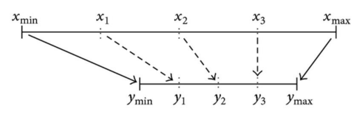
• Purpose: Scales values to the [0,1] range.
• Formula:
• Example: For , , → , .

2. Z-Score Standardization (Z分数标准化)

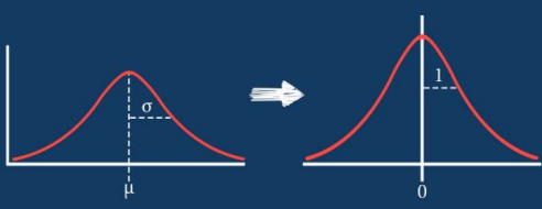
• Purpose: Scales values to a standard normal distribution (mean=0, variance=1).

• Formula:

• Example: For , , → .

Feature Selection & Engineering (特征选择与特征工程)

Feature Selection / Dimensionality Reduction (特征选择/降维)

“Too much data” slows down models—select only informative features: - Based on Missing Value Ratio (基于缺失值占比): Remove features with >50% missing values (no useful information). - Based on Low Variance (基于低方差): Remove features with near-constant values (variance < threshold, e.g., 0.01). They don’t contribute to predictions. - Based on High Correlation (基于高相关性): Remove one of two highly correlated features (correlation > 0.8). They carry redundant information.

Feature Engineering Techniques (特征工程技术)

Feature engineering creates new, powerful variables from raw data—this is where data scientists add the most value! 1. Scale Conversion (尺度转换): - Categorical → Numerical: One-hot encoding for multi-class variables (e.g., “color=red” → [1,0,0]). - Numerical → Categorical: Discretization (equal-width/equal-frequency bins, e.g., “age=35” → “adult”).

2. Ratio of Two Features (两特征比率):
   • Create meaningful metrics (e.g., “cost_per_sqft = property_price / square_footage” or “efficiency = actual_hours / standard_hours”).
3. Mathematical Transform (数学变换):
   • Box-Cox Transformation (Box-Cox变换): Converts non-normal data to approximate a Gaussian distribution.
     • Formula:
     • Use case: Improves model performance for algorithms assuming normality (e.g., linear regression).

---

Data processing is equal parts art and science—mastering these skills turns raw data into gold.
–Justin Zhang

欲知后事如何，且听下回分解